Source Code
First things first! You can get the code from the link below. Follow the instructions to download the Sponza art assets. Source Code
Recently, I was exploring different Motion Blur techniques being used in the industry. Now, I have decided to jot down the result of this research.
At first glance, I found several per-pixel motion blur approaches, but they did not impress me. To explain why I was not satisfied with the results, I need to give you some context!
Screen-space Motion Blur
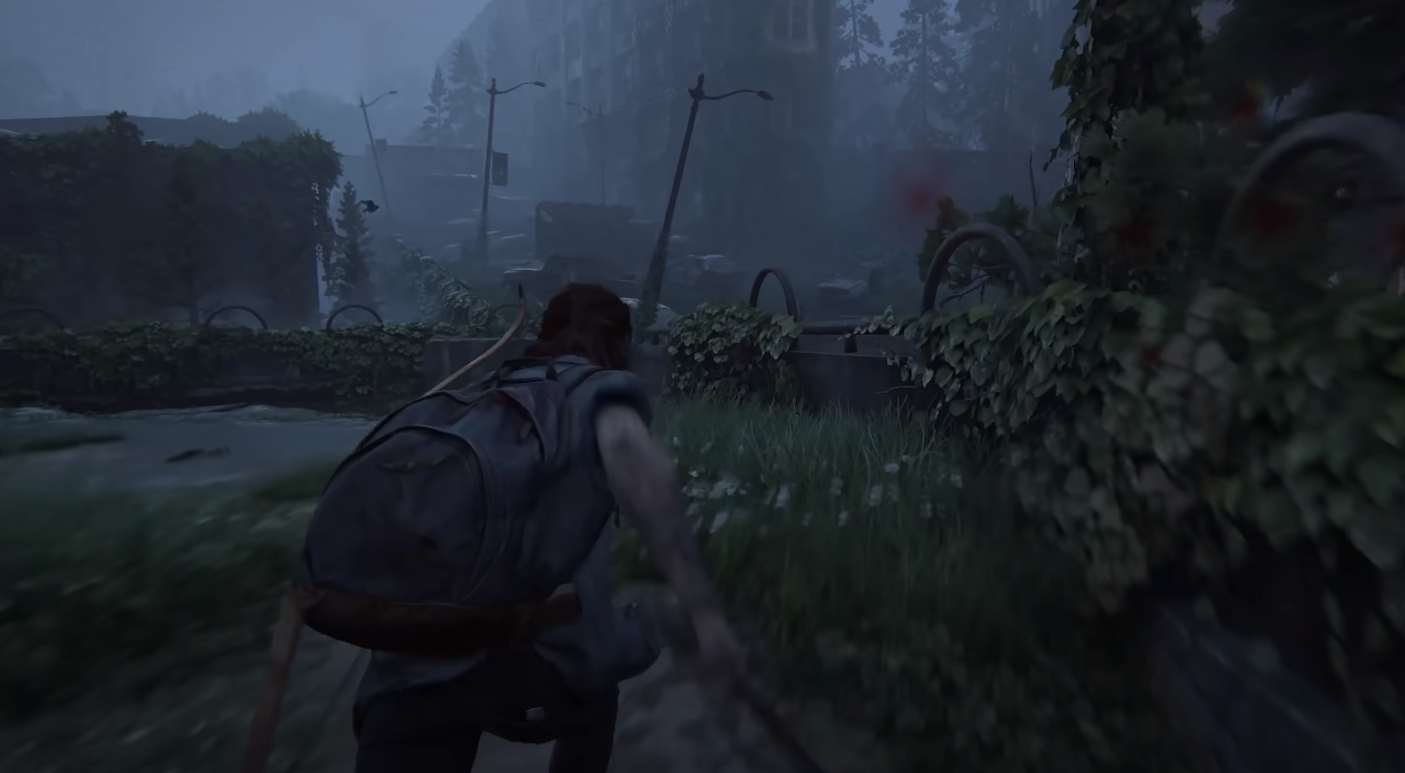
My main issue with the trivial approaches was that they would only take the camera motion into account. The problem with this approach is that the movement of the object would not make a discernible motion trail. Basically, in motion blur effects based on the camera’s position and orientation, one rendering pass would be dedicated to finding the difference in pixels’ position between the current frame and the previous one. The result of this render pass is stored in a render target, commonly called screen velocity vectors.
A Better Approach
As I was continuing my research, one method particularly caught my eye. It was called A Reconstruction Filter for Plausible Motion Blur by Prof. McGuire . I knew that this method is considered a bit old by now, but I also knew that it had proved its quality as it was used in many titles of its time.
Let’s first see how this method works:
Render the scene
Store the depth buffer. This is needed at the filter stage to preserve the sharpness of the edges.

- Create the velocity buffer based on the current and the previous objects’ world matrices, and store it as half-vectors.
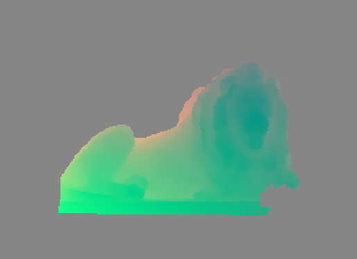
- Divide the velocity buffer into KxK tiles resulting a [Width/K]x[Height/K] buffer.
- Find the greatest velocity vector in each tile based on its length.
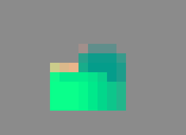
- Find the greatest velocity vector between all neighbors of each tile.
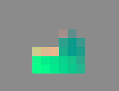
- Apply the blur filters.
function reconstruct(X, C, V, Z, NeighborMax):
   // Largest velocity in the neighborhood
   Let ~vN = NeighborMax[bX/kc]
   if ||~vN|| ≤ ε + 0.5px: return C[X] // No blur

   // Sample the current point
   weight = 1.0/||V[X]||; sum = C[X] · weight

   // Take S − 1 additional neighbor samples
   let j = random(−0.5, 0.5)
   for i ∈ [0, S), i 6= (S − 1)/2:
      // Choose evenly placed filter taps along ±~vN,
      // but jitter the whole filter to prevent ghosting
      t = mix (−1.0, 1.0,(i + j + 1.0)/(S + 1.0))
      let Y = bX + ~vN · t + 0.5pxc // round to nearest

      // Fore- vs. background classification of Y relative to X
      let f = softDepthCompare(Z[X], Z[Y])
      let b = softDepthCompare(Z[Y], Z[X])

      // Case 1: Blurry Y in front of any X
      αY = f · cone(Y, X, V[Y]) +

      // Case 2: Any Y behind blurry X;estimate background
      b · cone(X, Y, V[X]) +

      // Case 3: Simultaneously blurry X and Y
      cylinder(Y, X, V[Y]) · cylinder(X, Y, V[X]) · 2

      // Accumulate
      weight += αY ; sum += αY · C[Y]

   return sum/weight
Benefits
There are several benefits that this method brings to the table.
- Parallelism and cache efficiency
- A line-gathering filter
- Needs only to search along NeighborMax.
- Compute NeighborMax with two m-way parallel-gather operations on n/k2
- The entire algorithm is O(kn/m)-time
- Exhibits both high memory locality and parallel memory access.
- Keeps the edges sharp while blurring the moving objects
- Early out, when there is no movement going on in the radius of that pixel
If you want to learn more about this method, you can read the paper below in the references. Also, I need to mention that although there are many improvements that this method introduces, there exist more sophisticated and state-of-the-art solutions being used in AAA games. There are many great GDC and SIGGRAPH talks on this topic, so I am sure you can find them yourself.
An Optimized Implementation
Alright, enough with the introductions; now, it is time to talk about what I was able to do!
First of all, if this approach is considered to be a good one, then what is the problem? Well, even though today’s GPUs are way more powerful than the ones when this paper was first published (2012), it could be a good idea to implement the method in a more optimized way. So here is what I did to implement an optimized version of this method:
- Memory bandwidth is scarce, so we do not want to store all of our history buffers into render targets. We want to reduce GBuffer size and, consequently, reduce memory bandwidth usage. One Idea is to store the previous frame’s depth instead of position. This saves us some bytes as we can reconstruct the last frame’s position from the depth buffer and previous camera matrix.
- This whole approach is quite suitable for compute shaders. Yet, you may ask what advantages it has over our normal fragment/pixel shaders. Well, an architectural advantage of compute shaders for image processing is that they skip the ROP step. Also, the next point!
- To further optimize this method, we have to pay heed to our memory access pattern. In the Neighbor pass, we want to find the most dominant velocity vector between the neighbors. We are essentially accessing 8 neighbors, but these tiles share some neighbors. As a result, should we store the result of our texture fetches in the group shared memory (also called LDS), we can avoid the extra costly samples in the subsequent calls.
Future Work
There are more techniques to optimize the method further. For instance, instead of early exiting when velocity is lower than a threshold, we can have a pass where we classify the tiles and use IndirectDispatch for different complexities. Some tiles will be classified as early exit tiles, and some would be selected for further calculations. This way, we can save on our resources and regain some of the frame time.
Conclusion
Alright, finally, it is time to show some numbers. I implemented this project using The Forge rendering framework and ran it on an NVIDIA GTX 970. The results were as follows:
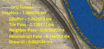
Do you see mistakes, typos, or have questions? Pleaes let me know!
References
- The Forge - Github
- Chapman J.: Per-Object Motion Blur
- McGuire, M., Hennessy, P., Bukowski, M., & Osman, B. (2012). A Reconstruction Filter for Plausible Motion Blur . Proceedings of the ACM SIGGRAPH Symposium on Interactive 3D Graphics and Games 2012 (I3D’12).
- Sponza model authored by Frank Meinl at Crytek .
- Sponza model acquired from McGuire Computer Graphics Archive .
